Drawing automorphisms

It can be helpful to see automorphisms rather than just read a description of them. To that end we introduce functions for rendering automorphisms as tree pair diagrams. The output looks best for automorphisms with a small arity (2–5) and a reasonable number of leaves.

Examples

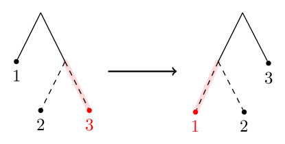
First we take a well-behaved automorphism. The solid carets are those belonging to both the domain and range trees. All other carets are dotted. Some edges are highlighted in red—these correspond to the repellers and attractors discussed by [SD10].

>>> from thompson import *
>>> x0 = standard_generator(0)
>>> plot(x0)
>>> forest(x0)

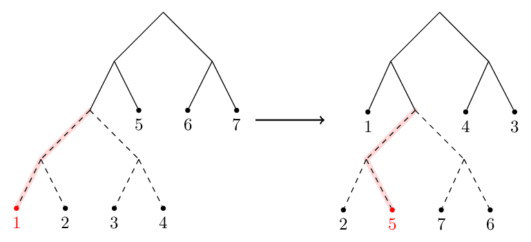
Discontinuities are fine too. Here’s example_4_17 for instance.

>>> pond = load_example('example_4_17')
>>> plot(pond, discontinuities=True)
>>> forest(pond)

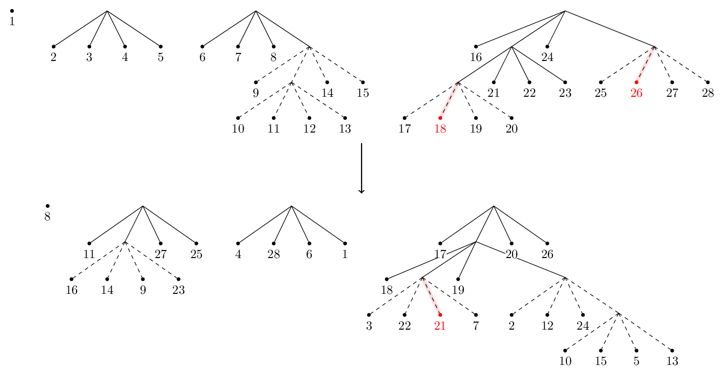
Let’s aim for something more chaotic. This example is complicated enough that the drawings don’t really give us much insight into the automorphism.

>>> random = random_automorphism() #different every time!
>>> plot(random)
>>> forest(random, horiz=False)

Drawing functions

thompson.drawing.display_file(filepath, format=None, scale=1.0, verbose=False)

Display the image at filepath to the user. This function behaves differently, depending on whether or not we execute it in a Jupyter notebook.

If we are not in a notebook, this function opens the given image using the operating system’s default application for that file.

If we are in a notebook, this returns an IPython object corresponding to the given image. If this object is the last expression of a notebook code block, the image will be displayed. The image is handled differently depending on its format, which must be specified when the function is called in a notebook. Only the formats ‘svg’ and ‘pdf’ are accepted.

Note

PDF files are displayed in a notebook as a rendered PNG. The conversion is made using the convert program provided by ImageMagick, which must be available on the PATH for this function to work with PDF files. The optional scale argument can be used to control how big the rendered PNG is.

Todo

use a Python binding to ImageMagick rather than just shelling out?

thompson.drawing.plot(*auts, dest=None, display=True, diagonal=False, endpoints=False, scale=1)

Plots the given automorphism s as a function \([0, 1] \to [0, 1]\). The image is rendered as an SVG using svgwrite.

Parameters:

• dest (str) – the destination filepath to save the SVG to. If None, the SVG is saved to a temporary file location.
• display (bool) – if True, automatically call display_file() to display the SVG to the user. Otherwise does nothing.
• diagonal (bool) – if True, draws the diagonal to highlight fixed points of aut.
• endpoints (bool) – if True, open and closed endpoints are drawn on the plot to emphasise any discontinuities that aut has.

Returns:

the filepath where the SVG was saved. If dest is None this is a temporary file; otherwise the return value is simply dest.

thompson.drawing.forest(aut, jobname=None, display=True, scale=1, **kwargs)

Draws the given Automorphism as a forest-pair diagram. The image is rendered as a PDF using the tikz graph drawing libraries and lualatex.

Parameters:

• jobname (str) – the destination filepath to save the PDF to. A file extension should not be provided. If None, the PDF is saved to a temporary file location.
• display (bool) – if True, automatically call display_file() to display the PDF to the user. Otherwise does nothing.
• scale (float) – In a Jupyter notebook, this controls the size of the rendered PNG image. See the note in display_file().

Returns:

the filepath where the PDF was saved. If dest is None this is a temporary file; otherwise the return value is simply jobname + ‘.pdf’.

Note

The graph drawing is done via a TikZ and LaTeX. The source file is compiled using lualatex, which must be available on the PATH for this function to work.

thompson.drawing.flow(aut, jobname=None, display=True)

thompson.drawing.forest_code(aut, name='', domain='wrt QNB', include_styles=True, horiz=True, LTR=True, standalone=True, draw_revealing=True)

Generate TikZ code for representing an automorphism aut as a forest pair diagram. The code is written to dest, which must be a writeable file-like object in text mode.

Parameters:

• name (str) – The label used for the arrow between domain and range forests. This is passed directly to TeX, so you can include mathematics by delimiting it with dollars. Note that backslashes are treated specially in Python unless you use a raw string, which is preceeded with an r. For instance, try name=r'\gamma_1
• domain (Generators) – By default, we use the minimal expansion of the quasi-normal basis as the leaves of the domain forest. This can be overridden by providing a domain argument.
• include_styles (bool) – Should the styling commands be added to this document?
• horiz (bool) – If True, place the range forest to the right of the domain. Otherwise, place it below.
• LTR (bool) – if True and if horiz is True, draw the domain tree to the left of the range tree. If horiz is True but LTR is false, draw the domain tree to the right of the range tree.
• standalone (bool) – If True, create a standalone LaTeX file. Otherwise just create TikZ code.
• draw_revealing (bool) – Should attractor/repeller paths be highlighted in red?